Evaluation

We use the evaluators for the evaluation of our models. Several evaluators can be used for the evaluation. The superclass :py:mod`kitcar_ml.utils.evaluation.evaluator` provides the interface for all evaluators. The evaluators can be called with the detections and groundtruths.

InterpolationEvaluator

The kitcar_ml.utils.evaluation.tutorial demonstrates how to use the evaluators. First, we fake a dataset and the detections to demonstrate the evaluator, with the following two functions. The following code demonstrates how to use an evaluator.

from kitcar_ml.utils.bounding_box import BoundingBox
from kitcar_ml.utils.evaluation.interpolation_evaluator import InterpolationEvaluator


def fake_dataset():
    """Simulate the dataset and create the groundtruth."""

    # Create 10 images with one bounding box each.
    bb = [[BoundingBox(x1=0, y1=0, x2=10, y2=10, class_label="1", confidence=1)]] * 10
    return bb


def fake_prediction():
    """Simulate a model and create predictions."""
    groundtruth = fake_dataset()

    # Only change the confidence
    groundtruth[0] = [BoundingBox(0, 0, 10, 10, "1", 0.8)]
    # Create a large bounding box
    groundtruth[1] = [BoundingBox(0, 0, 16, 14, "1", 0.7)]
    # Create two slightly large bounding boxes.
    groundtruth[2] = [BoundingBox(0, 0, 12, 12, "1", 0.7)]
    groundtruth[3] = [BoundingBox(0, 0, 8, 8, "1", 0.7)]
    return groundtruth


if __name__ == "__main__":
    # Initialize the evaluator.
    iou_thresholds = (0.3, 0.5, 0.8)
    interpolation_evaluator = InterpolationEvaluator(
        iou_thresholds, use_every_point_interpolation=False
    )

    # Load the dataset (for this tutorial we just fake them)
    groundtruths = fake_dataset()
    detections = fake_prediction()

    # Call the evaluator with the groundtruths and the detections.
    interpolation_evaluator(groundtruths, detections)

    # Output a summary of the evaluator.
    print(interpolation_evaluator)

    # Plot the calculated graphics. This can be different for every evaluator.
    interpolation_evaluator.plot_precision_recall_curves()

We initialize the evaluator with custom iou thresholds. The evaluator calculates the evaluation with the groundtruths and detections. Then a summary is printed and looks like this:

--------------
IoU 0.3
mAP: 1.0
--------------
IoU 0.5
mAP: 0.88
--------------
IoU 0.8
mAP: 0.7
--------------

The mean average precision(mAP) is calculated with the true and false positives. A detection is accepted, if the intersection over union ratio is higher than the threshold. That is why the mAP decreases with a higher iou threshold. We can see that the bounding box 1 and 2 have a higher iou than 0.5 and the bounding boxes 3 and 4 have a higher iou than 0.8.

We can also show the calculated interpolation in a plot. That creates these plots:

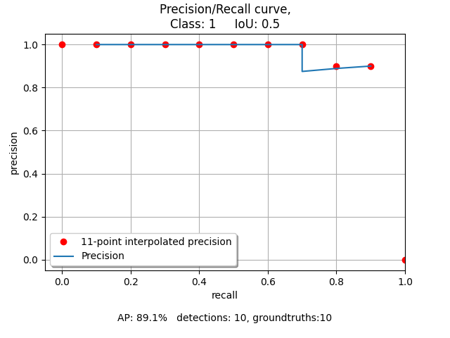
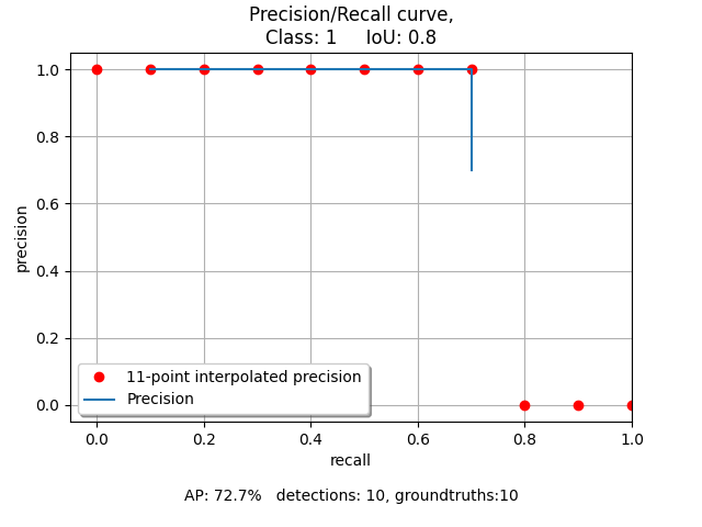
An interpolation is calculated for every iou threshold. Therefore this creates a plot for every iou threshold.

An explanation for IoU can be found at :ref: https://en.wikipedia.org/wiki/Jaccard_index

A larger example that generates more bounding boxes and changes the boxes more can be found in kitcar_ml.utils.evaluation.example.